Getting started

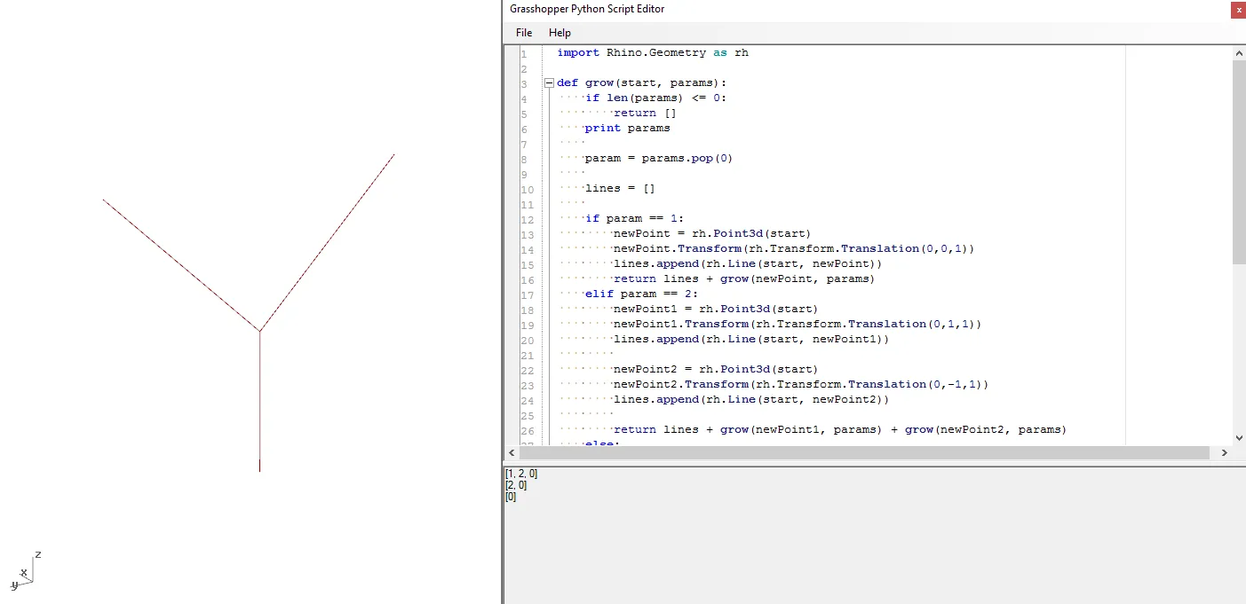
Let’s try this by creating a parametrized branching algorithm. Branching systems and other fractal geometries are commonly represented through recursive functions because they are self-similar, meaning that the same behavior is exhibited at various scales throughout the structure. For example, the branching of a set of large branches from the trunk of a tree is similar to the branching of a smaller set of branches from each of these branches. Here is the code for a basic branching algorithm in Python. You can paste it directly into a new Python node in Grasshopper.

import Rhino.Geometry as rh
def grow(start, params):
    if len(params) <= 0:
        return []
    
    param = params.pop(0)
    
    lines = []
    
    if param == 1:        
        newPoint = rh.Point3d(start)
        newPoint.Transform(rh.Transform.Translation(0,0,1))
        lines.append(rh.Line(start, newPoint))
        return lines + grow(newPoint, params)
    elif param == 2:
        newPoint1 = rh.Point3d(start)
        newPoint1.Transform(rh.Transform.Translation(0,1,1))
        lines.append(rh.Line(start, newPoint1))
        
        newPoint2 = rh.Point3d(start)
        newPoint2.Transform(rh.Transform.Translation(0,-1,1))
        lines.append(rh.Line(start, newPoint2))
        
        return lines + grow(newPoint1, params) + grow(newPoint2, params)
    else:
        return lines
a = grow(rh.Point3d(0,0,0), [1,2,0])

This code sequentially generates a branching structure based on a set of parameters which can be 0, 1, or 2. The grow() function takes in a starting point and creates zero, one, or two new branches based on the first parameter in a set. It then calls the grow() function again with the end of each new branch as the starting point and the reduced parameter list. The output of the grow function is a list of lines representing the branches. Let’s step through the function calls using an example set of parameters [1,2,0] to see how it works.

The first time we call the grow function we pass in a new point at the origin [0,0,0] along with the full set of parameters. At this point, the length of the parameter list is 3, so the termination criteria is not met and the function continues. Next the function pops the first parameter from the list and stores it in the param variable. It also creates an empty list called ‘lines’ to store the geometry of the branches it creates.

Now the function encounters a set of conditionals which do different things depending on the value of the current parameter. If the parameter value is ‘1’ it makes one new branch by creating a new point as a copy of the start point:

newPoint = rh.Point3d(start)

It then moves that point one unit in the z direction to create a vertical branch:

newPoint.Transform(rh.Transform.Translation(0,0,1))

It then creates a new line between the start and new point and appends it to the lines list:

lines.append(rh.Line(start, newPoint))

Finally, it returns this set of new lines, added to the set of lines from the next call to grow(), which takes in the new point as its starting point and the reduced set of parameters.

The behavior for a parameter value of '2' is similar except we now create two diagonal branches instead of one vertical one and call the grow() function twice in the return statement. At first it might seem that calling the function twice in one line would pass the same parameter values to both new branches, so that we would end up with more branches that starting parameter values. In fact, when we use variable names in Python we are actually using references to the variable stored somewhere in memory, which means that all the function calls are actually interacting with the same exact list. This means that when one function pops a value out of the list, the list is affected for all subsequent functions, even if they are called later on the same line.

In this example the first call to the grow() function pops one of the parameters from the list so it is already reduced when the second grow() function is executed later in the line. In this case this is what we want since we only want each parameter to be considered once. If we actually wanted to pass the same exact parameter list to both function calls we would first have to make a copy of the list. To make sure each parameter is only being used once we can print the values in the parameter list at the beginning of each function call:

The final conditional in the function is an else statement that captures any other possible parameter value and results in the return of an empty list. This includes the parameter 0 which we expect to terminate the branching procedure. Although we could have programmed the behavior for our expected inputs of 0, 1, and 2 through their own explicit conditionals, it is good practice to nest all of the conditions together using elif statements and have a final else condition at the end to capture all other cases. This provides a fail-safe termination condition that ensures that the recursive function will always terminate even if you enter an unexpected value by accident.

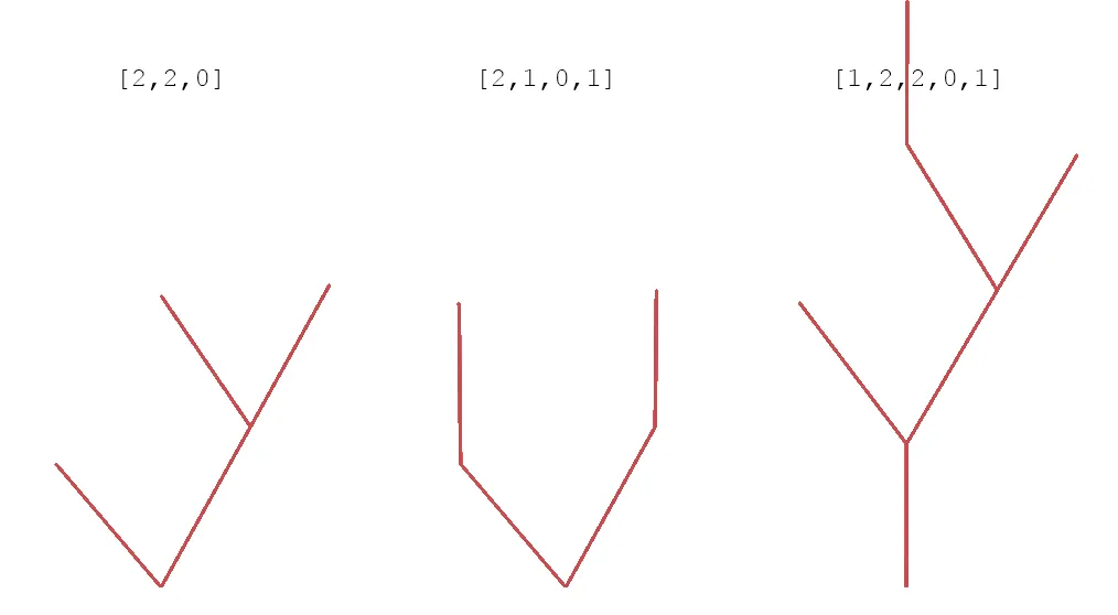
For our parameter set of [1,2,0], the first call to grow() generates one vertical branch and calls grow() again. The second call creates two diagonal branches and calls grow() two more times. The first of these calls returns an empty list because the parameter is '0'. The second call also returns an empty list because there are no more parameters in the list. This results in the structure seen above. Here are some other possible structures based on different sets of input parameters. Note that the '0' parameter has the effect of stopping any branching path, so any sequence starting with '0' will produce no branches since the behavior is stopped at the first step.

This example shows the power of recursive functions in defining complex forms based on a small set of abstract parameters. However, the use of recursion is not restricted only to branching problems. In fact any system can be implemented using recursive functions as long as it can be described based on smaller versions of itself. In a later exercise, we will see how a similar kind of recursive algorithm can be used to subdivide a given space into several other spaces.

CHALLENGE

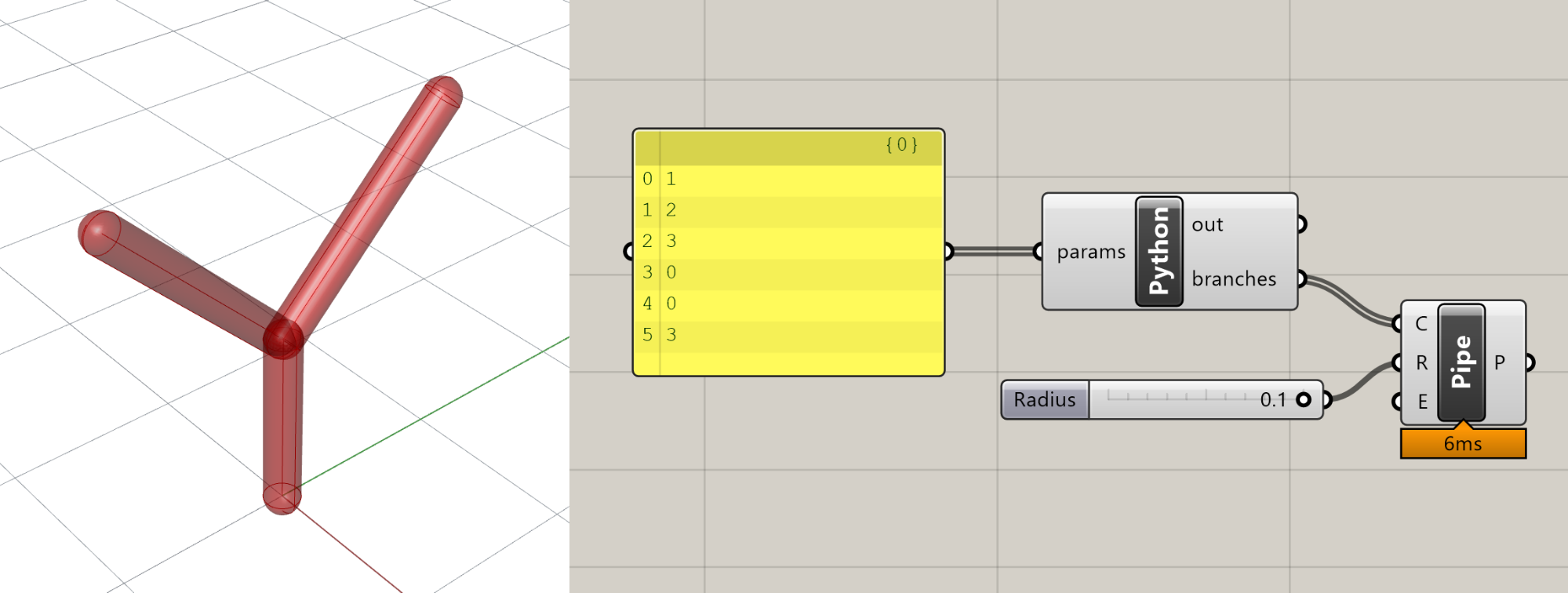
Download the starting Grasshopper file and open it up in a blank Rhino and Grasshopper file. The model’s Python component contains the definition of the tree model developed in class. It also includes a list of input parameters that are passed into the Python component from a Panel component, and uses a Pipe component to visualize the branch geometry as closed cylinders.

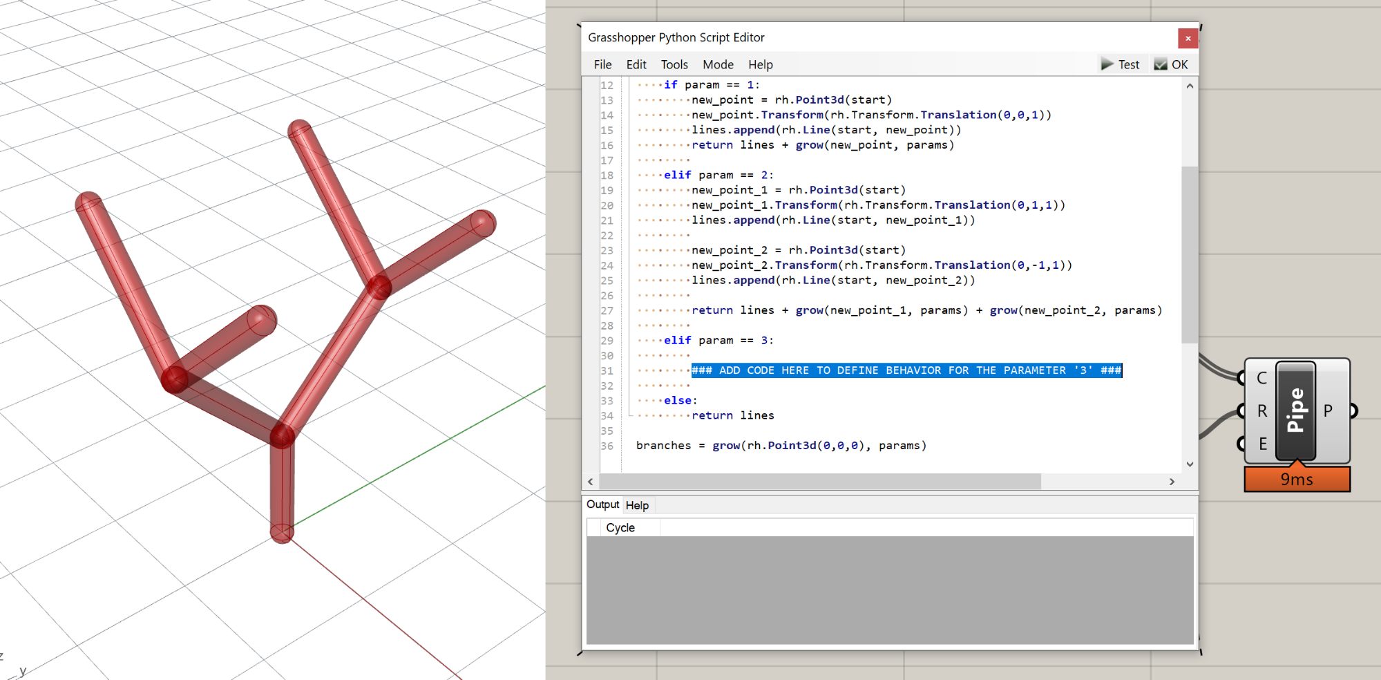
Your task is to add additional code within the Python script to define a new branching behavior for the ‘3’ parameter that creates the branching seen in the screenshot below. You should only add code within the elif param == 3: code block starting on line 35 of the Python script. You should not need to modify anything else about the code, the Grasshopper definition, or the set of parameters.

Once you’ve generated the proper branching, take a screenshot showing the geometry in Rhino and the code you added. Name the file with your UNI and/or name, and upload to: https://www.dropbox.com/request/gDCkyn9KGWiOJ0SyqFjD

HINT: Currently, the behavior for the parameter '3' is the same as for '0' or any other undefined parameter. It simply returns the empty list, stopping the branching at the current point. To get the branching result shown, you should add a logic similar to the one for the parameter '2', but generating two branches going in the 'x' instead of the 'y' direction.

Conclusion

In this exercise, we created a recursive function that can generate a branching tree based on a set of parameters.